Maple Programming
Graphing
How to plot a set of data points and a function

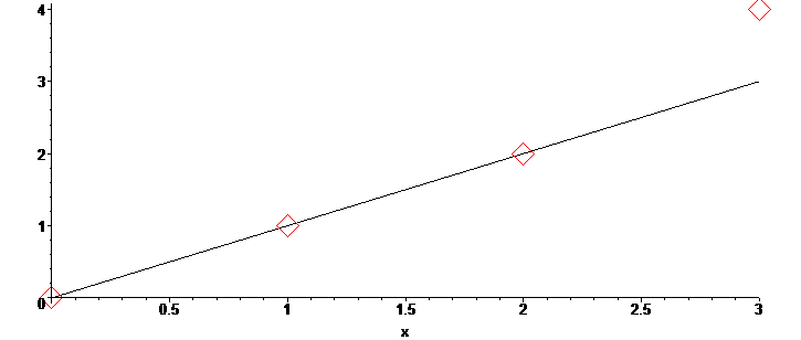
data:=[[0,0],[1,1],[2,2],[3,4]];
plot ([data,f(x)],x=0..3,style=[point,line],symbolsize=40,color=[red,black]);
That plots the [x,y] coordinates as 'data' and also plots the function f(x)
or
if you want to generate data to plot from a sequence, seq() can be used to output [x,y] pairs:
data:=[seq([n,f(n)],n=1..10)];
plot ([data],style=point,thickness=20);
This can be useful to mark specific data-points when plotting along side a line defined by a continuous function, for example.
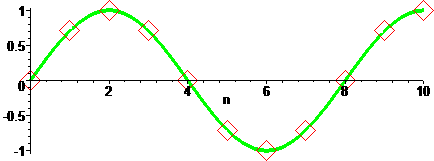
data:=[seq([n,sin(n/4*Pi)],n=0..10)];
plot ([data,sin(n*Pi/4)],n=0..10,style=[point,line],symbolsize=40,thickness=20);

The definition for the data in terms of seq(function) can be called directly from the plot function.
plot ([seq([x,f(x)],x=1..40)],style=point,thickness=20);
or
When the data has to be loaded from a file and is formatted as a sequential
list of y-data, it can be convenient to construct the x,y pairs from two
separate arrays containing only
ydata:=[1,2,3,4];
xdata:=[seq(i,i=1..nops(ydata))];
pair:=(x,y)->[x,y];
data:=zip(pair,xdata,ydata);
plot([data]);
Solving a system of differential equations
sadadasd
sys_ode:= diff(A(t),t)=(2*k2-k1)*A(t)*B(t)-k2*A(t)^2, diff(B(t),t)=-k1*A(t)*B(t); ics:=A(0)=2,B(0)=1; dsolve([sys_ode,ics]);
Output data to text files
Writing to output files, such as csv files that can be loaded into Excel
fd:=fopen("c:/users/resospace/outputfile.txt", WRITE);

fprintf (fd,"%s,%s,%s,%s\n","column-A","column-B","Column-C","blank");

for x from 1.5 by 0.01 to 2.5 do
   fprintf (fd,"%E,%E,%E,%E\n",x,x*2,x*3,0);
end do;
fclose(fd);
or much more simply,
fd:=fopen("c:/users/resospace/outputfile.txt", WRITE);

writedata(fd,data);

fclose(fd);
Reading a tab delimited csv file
How to import data where 2 is the number of columns and the file does not
contain column headers.
fh:=fopen("C:/Users/resospace/Desktop/tabdelim.csv", READ);

data:=readdata(fh,2);

fclose(fh);
Some 3d graphing
and why not
restart;
 with(plots):
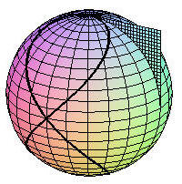
 sphere1:=plot3d([sin(f)*cos(t),sin(f)*sin(t),cos(f)],f=0..Pi,t=0..2*Pi):
 curve1:=spacecurve([(cos(t))^2,cos(t)*sin(t),sin(t)], t=0..2*Pi,color=black,thickness=3):

 plane1:=plot3d([0,v,u],u=0..1,v=0..1):
 display([sphere1,curve1,plane1],scaling=constrained);

and why not
with(plots):
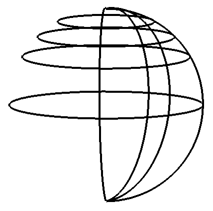
m1:=spacecurve([sin(f), 0, cos(f)],f=0..Pi):
m2:=spacecurve([1/2*sin(f)*2^(1/2), 1/2*sin(f)*2^(1/2), cos(f)],f=0..Pi):
m3:=spacecurve([1/2*sin(f), 1/2*sin(f)*3^(1/2), cos(f)],f=0..Pi):
m4:=spacecurve([0, sin(f), cos(f)],f=0..Pi):
m5:=spacecurve([1/2*cos(t), 1/2*sin(t), 1/2*3^(1/2)],t=0..2*Pi):
m6:=spacecurve([1/2*2^(1/2)*cos(t), 1/2*2^(1/2)*sin(t), 1/2*2^(1/2)],t=0..2*Pi):
m7:=spacecurve([cos(t), sin(t), 0],t=0..2*Pi):
m8:=spacecurve([1/2*3^(1/2)*cos(t), 1/2*3^(1/2)*sin(t), 1/2],t=0..2*Pi):
display(m1,m2,m3,m4,m5,m6,m7,m8,color=black,thickness=4);

Misc
Random files: